
Heat Waves
Published:
The recent days have seen quite a heat wave hit Europe, and especially Bulgaria. At the same time, I cam upon this article in the Financial Times, arguing that lack of air conditioning in Europe vis-a-vis the United States up to twice higher death rates on days with temperatures exceeding 28 degrees Celsium.
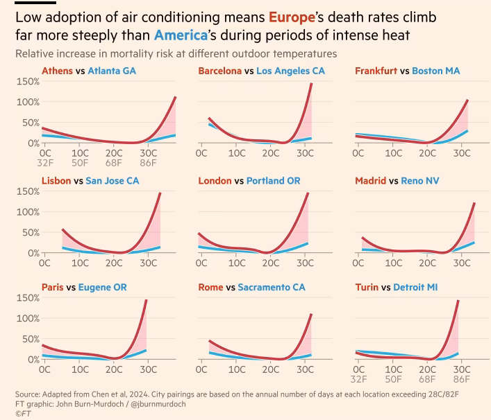
I have never seen an excess heat deaths graph for Bulgaria, so naturally, I set up to make one. The time budget I gave myself was one afternoon, so let’s see how far we can get.
The academic reference for the chart above is Chen et al. 2024, and while I won’t follow their approach 1:1 it is mostly the same idea. We are going to try to fit a (non-linear) mortality model with a spline temperature predictor along with some demographic controls and see what we get as a result.
Input Data
We need three sources of data: deaths, population (so we can estimate death rates), and temperature. The lower the granularity, the better.
Starting with deaths, NSI publishes weekly totals, broken down by region, gender, and age group. Population estimates are also available at a similar granularity, but only on an annual basis. Still, for the current purposes it will do.
The European Climate Assessment project provides daily temperature data on a 10km grid across Europe. Specifically, I am going to use the tx_ens_mean_0.1deg_reg_v31.0e.nc dataset, which contains data on maximum daily temperatures.
Data Cleaning
The temperature data was in the .ns format, which I haven’t encountered before. Since the file is quite large, we can filter based on geographical coordinates and dates and read only the part that we need. After some formatting efforts, we get it into a tidy format:
read_temperature <- function(
  file_path = "data/tg_ens_mean_0.1deg_reg_v31.0e.nc",
  from_date = as.Date("2015-01-01"),
  measure = "tx"
) {
  temperature_file <- nc_open(file_path)

  print(temperature_file)

  longitude <- ncvar_get(temperature_file, "longitude")
  latitude <- ncvar_get(temperature_file, "latitude")
  time_vals <- ncvar_get(temperature_file, "time")
  time_dates <- as.Date(time_vals, origin = "1950-01-01") # "days since 1950-01-01 00:00"

  bulgaria_coords <- list(
    lat_min = 41, lat_max = 44.5, lon_min = 22, lon_max = 29
  )

  # Find indices for Bulgaria's spatial extent
  lon_indices <- which(
    (longitude >= bulgaria_coords$lon_min) & (longitude <= bulgaria_coords$lon_max)
  )
  lat_indices <- which(
    latitude >= bulgaria_coords$lat_min & latitude <= bulgaria_coords$lat_max
  )
  # Find temporal indices for 2015 onwards
  time_indices <- which(time_dates >= from_date)

  # Extract data for Bulgaria from 2015 onwards
  bulgaria_temp <- ncvar_get(
    temperature_file, measure,
    start = c(min(lon_indices), min(lat_indices), min(time_indices)),
    count = c(length(lon_indices), length(lat_indices), length(time_indices))
  )

  bulgaria_lon <- longitude[lon_indices]
  bulgaria_lat <- latitude[lat_indices]
  bulgaria_dates <- time_dates[time_indices]

  temperature <- crossing(
    i = seq_along(bulgaria_lon),
    j = seq_along(bulgaria_lat),
    k = seq_along(bulgaria_dates)
  ) %>%
    transmute(
      lon = bulgaria_lon[i],
      lat = bulgaria_lat[j],
      date = bulgaria_dates[k],
      t = bulgaria_temp[cbind(i, j, k)]
    )
}

temperature <- read_temperature("data/tx_ens_mean_0.1deg_reg_v31.0e.nc")
Since we have weekly deaths data, we will also have to aggregate the temperature to a weekly average (of daily max values). Also, since the temperature data is on a grid, we will have to decide exactly which values to use for every region in the NSI data.
One approach would be to average all observations within a given region. That wouldn’t be ideal though, as the population is not uniformly spread over the territory of the given region. For example, for Blagoevgrad we would be taking some measurements in the high mountains, where basically nobody lives.
Instead, I decided to just take the grid square closest to the biggest population center in each region and use that as the measurement for the entire region. Not ideal, but it should be widely representative of the temperatures the majority of the region’s populations experiences.
regional_cities <- bind_rows(read_json("data/bulgaria_regional_cities.json"))

grid_points <- temperature %>%
  distinct(lat, lon)

closest_grid_point <- map(regional_cities$name, function(city) {
  city_lat = regional_cities$lat[regional_cities$name == city]
  city_lon = regional_cities$lon[regional_cities$name == city]
  grid_points %>%
    mutate(
      dist = haversine_dist(
        lat, lon,
        city_lat, city_lon
      )
    )%>%
    arrange(dist) %>%
    slice(1) %>%
    select(lat, lon) %>%
    mutate(region = city)
}) %>%
    bind_rows()
With that out the way, we can go ahead with joining all data together. Only thing left to do is accounting for the slightly different age groupings in the population and mortality data from NSI:
population <- read_csv("data/population.csv")
deaths <- read_csv("data/mortality.csv")

mortality <- deaths %>%
  pivot_longer(
    cols = starts_with("y"),
    names_to = "date_",
    values_to = "deaths"
  ) %>%
  mutate(
    year = as.numeric(str_extract(date_, "(?<=y)\\d{4}")),
    week = as.numeric(str_extract(date_, "(?<=_w)(\\d+)")),
    gender = ifelse(str_detect(date_, "female"), "female", "male"),
    date = make_date(year) + weeks(week - 1)
  ) %>%
  arrange(
    region, gender, age_group, date
  ) %>%
  inner_join(
    population %>%
      mutate(
        age_group = ifelse(age_group %in% c("0", "1-4"), "0-4", age_group),
        age_group = ifelse(age_group %in% c("90-94", "95-99", "100+"), "90 +", age_group)
      ) %>%
      group_by(year, region, age_group) %>%
      summarise(male = sum(male, na.rm = T), female = sum(female, na.rm = T)) %>%
      pivot_longer(
        cols = c("male", "female"),
        names_to = "gender",
        values_to = "population"
      ),
    by = c("year", "region", "age_group", "gender")
  ) %>%
  select(
    region, date, age_group, gender, population, deaths
  )


# join mortality and temperature figures ----------------------------------
mortality <- mortality %>%
  left_join(
    closest_grid_point, by = "region"
  ) %>%
  left_join(
    temperature %>%
      mutate(
        year = year(date),
        week = week(date)
      ) %>%
      group_by(lon, lat, year, week) %>%
      summarise(
        t = mean(t, na.rm = T)
      ) %>%
      mutate(
        date = make_date(year) + weeks(week - 1)
      )
  ) %>%
  mutate(
    death_rate_1w = deaths/population * 1000 # per 1000 people
  )
Finally, since heat deaths are likely to disproportionally affect older people, we can focus only on the subset of the population in retirement age:
old_ages  <- c(
  "90 +",
  "85-89",
  "80-84",
  "75-79",
  "70-74",
  "65-69"
)
Model
For the modelling part we will use a Poisson generalized additive model. Namely:
\begin{equation} Y_i = Poisson(\mu_i, \phi) \end{equation}
where $Y_i$ is deaths for a given week-gender-age-region group. $\mu_i$ in turn is:
\begin{equation} log{\mu_i}=log{N_i} + f(t_i) + controls \end{equation}
$N_i$ is the population, and $f()$ is a spline function. The death rate is thus:
\begin{equation} \lambda_i = \frac{\mu_i}{N_i} = exp\left[f(t_i)+controls\right] \end{equation}
Therefore the exponent of any coefficient (or a given value of the spline function $f()$) from the model below should be interpreted as a relative multiplicative change in death rates, holding all controls fixed.
Estimation
Fitting the model with the bam package, we have:
model_df <- mortality %>%
  rename(temp = t) %>%
  mutate(
    date_num = as.numeric(date), # for long term trend
    doy      = yday(date), # seasonal trend
    age_group = as.factor(age_group),
    gender = as.factor(gender),
    region = as.factor(region),
    year = as.factor(year(date)),
    month = as.factor(month(date))
  )

set.seed(20250730)

g_simple <- bam(
  deaths ~
    s(temp, k = 9, bs = "cs") + # non‑linear temperature-response
    year + # yearly average
    month + # seasonal pattern
    age_group + # control for age
    gender + # control for gender
    region, + # regional dummies
    offset(log(population)), # we are modelling raw counts
  family = quasipoisson(link = "log"),
  data   = model_df %>% filter(age_group %in% old_ages),
  method = "fREML"
)

g_death <- bam(
  deaths ~
    s(temp, k = 9, bs = "cs") + # non‑linear temperature-response
    s(date_num, k = 15, bs = "cs") + # smooth long‑term trend (multi‑year)
    s(doy, bs = "cc", k = 12) + # cyclic seasonal pattern inside each year
    age_group + # control for age
    gender + # control for gender
    s(region, bs = "re"), + # regional random effects for shrinking
    offset(log(population)), # we are modelling raw counts
  family = quasipoisson(link = "log"),
  data   = model_df %>% filter(age_group %in% old_ages),
  method = "fREML"
)
We control for overall long-term trends, seasonal pattern, age, gender, and region. I have included two versions of the model. The simpler one just includes fixed effects dummies for all controls, while the more “complicated” one incorporates more spline funcitons and random effects. The results are not meaningfully different.
summary(g_death)
Family: quasipoisson
Link function: log

Formula:
deaths ~ s(temp, k = 9, bs = "cs") + s(date_num, k = 15, bs = "cs") +
    s(doy, bs = "cc", k = 12) + age_group + gender + s(region,
    bs = "re")

Parametric coefficients:
                Estimate Std. Error t value Pr(>|t|)
(Intercept)     1.242184   0.097891  12.690  < 2e-16 ***
age_group70-74  0.233220   0.004274  54.568  < 2e-16 ***
age_group75-79  0.352411   0.004198  83.942  < 2e-16 ***
age_group80-84  0.500775   0.004114 121.731  < 2e-16 ***
age_group85-89  0.405932   0.004271  95.038  < 2e-16 ***
age_group90 +  -0.039554   0.004987  -7.931 2.19e-15 ***
gendermale     -0.058248   0.002407 -24.197  < 2e-16 ***
---
Signif. codes:  0 ‘***’ 0.001 ‘**’ 0.01 ‘*’ 0.05 ‘.’ 0.1 ‘ ’ 1

Approximate significance of smooth terms:
               edf Ref.df       F p-value
s(temp)      7.140      8  4839.8  <2e-16 ***
s(date_num) 13.908     14  1036.5  <2e-16 ***
s(doy)       9.631     10   295.8  <2e-16 ***
s(region)   26.994     27 11351.3  <2e-16 ***
---
Signif. codes:  0 ‘***’ 0.001 ‘**’ 0.01 ‘*’ 0.05 ‘.’ 0.1 ‘ ’ 1

R-sq.(adj) =  0.687   Deviance explained = 63.6%
fREML = 4.5825e+05  Scale est. = 10.858    n = 175392
Heat and Mortality
We can finally answer the original question and examine the relationship between heat and mortality:
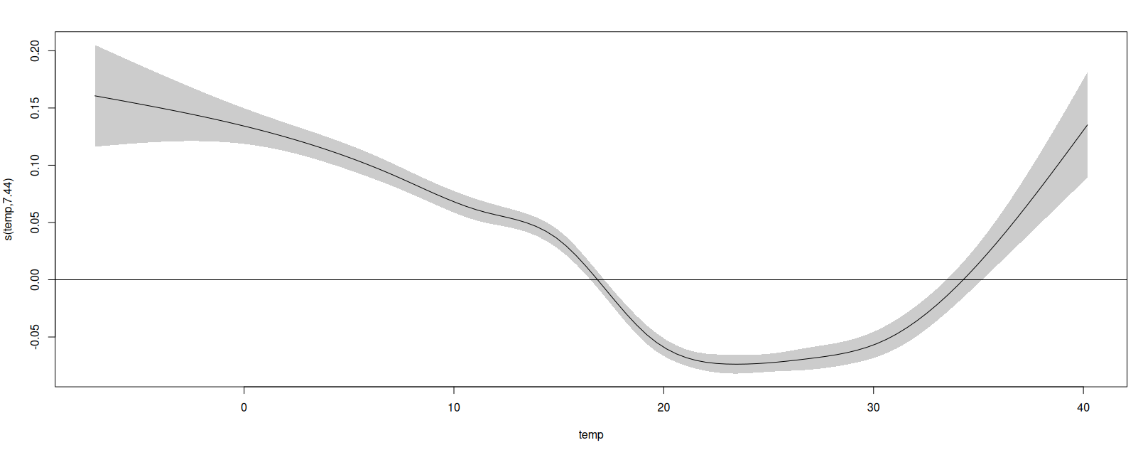
We can see that according to the model both high and low temperatures are associated with elevated mortality, while the 20-30 degree range has the lowest relative death rates (remember, we are taking into account seasonal effects separately).
The way to read this is that a week with an average daily high of 40 degrees is associated with about 23% more deaths than a week with an average weekly high of 30 degrees ($\frac{exp(t(40))}{exp(t(30))}=\frac{exp(0.14)}{exp(-0.07)}$). Since the average weekly death rate for this age group in the data is $1.157$ and there are just over 1.5 million pensioners in Bulgaria, this all adds up to about $400$ extra weekly deaths when we have averages of above 40-degrees.
While the relationship is clearly there and is significant, the magnitude seems somewhat weaker than the ones from Chen et al. But since it’s 17:20, it means my time budget is spent, so we’ll leave it at that for now.